[1]:
import arviz as az
import matplotlib.patches as mpatches
import matplotlib.pyplot as plt
import numpy as np
import pandas as pd
import pymc as pm
from sklearn.preprocessing import StandardScaler

from learn_data import DATA
from learn_data.regression import plot_corner, scaled_parameters_to_original

RANDOM_SEED = 42
"""Random seed for reproducibility."""
[1]:
'Random seed for reproducibility.'
5. Case Study: Absorption Coefficient
Thompson, M.A., P.A. Sossi, D.J. Bower, A. Shahar, C. Liebske, and J. Allaz (2025), Water solubility in silicate melts: The effects of melt composition under reducing conditions and implications for nebular ingassing on rocky planets, Chemical Geology, 695, 123048, doi: https://doi.org/10.1016/j.chemgeo.2025.123048
Read the data.
[2]:
filename = DATA.joinpath("absorption_coefficient/MolarAbsvsOpBasicity_forFitting.csv")
data = pd.read_csv(str(filename))

# Extract the predictor and response variables, along with their uncertainties, from the DataFrame.
predictor = data["OpBasic"].to_numpy()
response = data["Eps_m2mol"].to_numpy()
response_std = data["Eps_m2mol_unc"].to_numpy()
Scale the data.
[3]:
# Create a stacked array of the predictor and response variables, with shape (n_samples, 2).
stacked_values = np.stack((predictor, response), axis=1)

# Create a stacked array of the uncertainties, with zeros for the predictor variable (since we
# assume no uncertainty in the predictor).
stacked_stds = np.stack((np.zeros_like(predictor), response_std), axis=1)

# Create the scaled data
standard_scaler = StandardScaler()
stacked_values_scaled = standard_scaler.fit_transform(stacked_values)
stacked_stds_scaled = stacked_stds / standard_scaler.scale_

# We can also extract the scaled predictor and response variables, along with their uncertainties,
# into separate variables. This makes the code more readable. Note this produces 1-D arrays.
x_scaled = stacked_values_scaled[:, 0]
y_scaled = stacked_values_scaled[:, 1]
y_std_scaled = stacked_stds_scaled[:, 1]
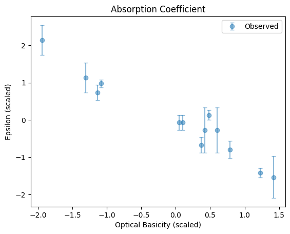
Plot the relationship.
[4]:
fig, ax = plt.subplots()
ax.errorbar(x_scaled, y_scaled, yerr=y_std_scaled, fmt="o", label="Observed", capsize=3, alpha=0.5)
ax.set_xlabel("Optical Basicity (scaled)")
ax.set_ylabel("Epsilon (scaled)")
title = "Absorption Coefficient"
ax.set_title(title)
ax.legend()
[4]:
<matplotlib.legend.Legend at 0x7f9fb1a34ad0>
Run the Bayesian model.
[5]:
with pm.Model() as model:
    # Define the prior distributions for the slope and intercept parameters.
    slope = pm.Normal("slope", mu=0, sigma=1)
    intercept = pm.Normal("intercept", mu=0, sigma=1)

    # The expected value of y for each x, given the parameters (the model).
    # This is just a linear model: y = mx + c, where m is the slope and c is the intercept.
    mu = slope * x_scaled + intercept

    # Define the likelihood: how likely the observed data are, given the model parameters.
    # We assume the observed y values are normally distributed around mu, with noise given by
    # y_std.
    y_obs = pm.Normal("y_obs", mu=mu, sigma=y_std_scaled, observed=y_scaled)

    # Sample from the posterior distribution using MCMC.
    idata = pm.sample(2000, tune=1000, return_inferencedata=True, random_seed=RANDOM_SEED)
Initializing NUTS using jitter+adapt_diag...
Sequential sampling (2 chains in 1 job)
NUTS: [slope, intercept]
/home/docs/checkouts/readthedocs.org/user_builds/learn-data/envs/latest/lib/python3.13/site-packages/rich/live.py:2
60: UserWarning: install "ipywidgets" for Jupyter support
  warnings.warn('install "ipywidgets" for Jupyter support')
Sampling 2 chains for 1_000 tune and 2_000 draw iterations (2_000 + 4_000 draws total) took 2 seconds.
We recommend running at least 4 chains for robust computation of convergence diagnostics
Compute the data required for the HDI calculation.
[6]:
with model:
    pm.sample_posterior_predictive(idata, extend_inferencedata=True, random_seed=RANDOM_SEED)
Sampling: [y_obs]
/home/docs/checkouts/readthedocs.org/user_builds/learn-data/envs/latest/lib/python3.13/site-packages/rich/live.py:2
60: UserWarning: install "ipywidgets" for Jupyter support
  warnings.warn('install "ipywidgets" for Jupyter support')
Extract the samples of the slope and intercept from the sampling process and compute a point estimate.
[7]:
# Extract samples for slope and intercept
m_samples_scaled = idata["posterior"]["slope"].stack(samples=("chain", "draw")).values
c_samples_scaled = idata["posterior"]["intercept"].stack(samples=("chain", "draw")).values

# Marginal median estimate for slope and intercept
# This is computationally faster than computing the joint distribution MAP estimate, although it
# does not capture the covariance between slope and intercept. Nevertheless, it is a common point
# estimate used in Bayesian regression and for simple linear regression it often gives similar
# results to the joint MAP estimate.
median_m_scaled = np.median(m_samples_scaled)
median_c_scaled = np.median(c_samples_scaled)
median_m, median_c = scaled_parameters_to_original(
    median_m_scaled, median_c_scaled, standard_scaler
)

print('"Best fitting" parameters for the linear regression model:')
print(f"Scaled median estimate: Slope (m) = {median_m_scaled}, Intercept (c) = {median_c_scaled}")
print(f"Median estimate: Slope (m) = {median_m}, Intercept (c) = {median_c}")
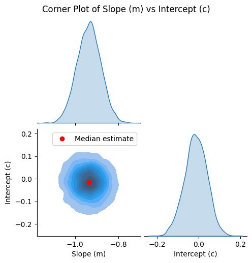
"Best fitting" parameters for the linear regression model:
Scaled median estimate: Slope (m) = -0.9356039184443918, Intercept (c) = -0.014772859800506572
Median estimate: Slope (m) = -15.091665498168044, Intercept (c) = 15.363653462750637
Plot the corner plot.
[8]:
g = plot_corner(m_samples_scaled, c_samples_scaled)

# Plot the median estimate on the lower left plot
ax = g.axes[1, 0]
ax.plot(median_m_scaled, median_c_scaled, "ro", label="Median estimate")
ax.legend()
[8]:
<matplotlib.legend.Legend at 0x7f9f99080a50>
Plot the observations and regression result.
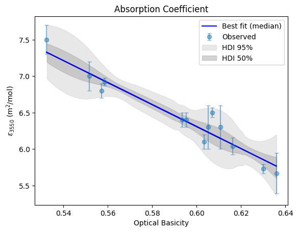
[9]:
y_pp_scaled = idata["posterior_predictive"]["y_obs"].stack(samples=("chain", "draw")).values
# Convert the posterior predictive samples back to original units for plotting
y_pp = y_pp_scaled.T * standard_scaler.scale_[1] + standard_scaler.mean_[1]  # type: ignore

fig, ax = plt.subplots()
ax.errorbar(
    predictor, response, yerr=response_std, fmt="o", label="Observed", capsize=3, alpha=0.5
)

# Add "best" fit line using the point estimates for slope and intercept
y_map_fit = predictor * median_m + median_c
ax.plot(predictor, y_map_fit, "b-", label="Best fit (median)")

# Plot the HDI regions
az.plot_hdi(
    predictor, y_pp, hdi_prob=0.95, fill_kwargs={"alpha": 0.5, "color": "lightgrey"}, ax=ax
)
az.plot_hdi(predictor, y_pp, hdi_prob=0.5, fill_kwargs={"alpha": 0.5, "color": "darkgrey"}, ax=ax)

# Manually add legend entries for HDI regions
handles, labels = ax.get_legend_handles_labels()
hdi_95_patch = mpatches.Patch(color="lightgrey", alpha=0.5, label="HDI 95%")
hdi_50_patch = mpatches.Patch(color="darkgrey", alpha=0.5, label="HDI 50%")
handles += [hdi_95_patch, hdi_50_patch]
labels += ["HDI 95%", "HDI 50%"]

ax.legend(handles=handles)  # Update legend with HDI entries

ax.set_xlabel("Optical Basicity")
ax.set_ylabel(r"$\epsilon_{3550}$ (m$^{2}$/mol)")
title = "Absorption Coefficient"
ax.set_title(title)
/home/docs/checkouts/readthedocs.org/user_builds/learn-data/envs/latest/lib/python3.13/site-packages/arviz/plots/hdiplot.py:166: FutureWarning: hdi currently interprets 2d data as (draw, shape) but this will change in a future release to (chain, draw) for coherence with other functions
  hdi_data = hdi(y, hdi_prob=hdi_prob, circular=circular, multimodal=False, **hdi_kwargs)
[9]:
Text(0.5, 1.0, 'Absorption Coefficient')