4. Bayesian Parameter Estimation II

# SPDX-FileCopyrightText: 2026 Dan J. Bower <dbower@eaps.ethz.ch>
#
# SPDX-License-Identifier: GPL-3.0-or-later

import arviz as az
import matplotlib.patches as mpatches
import numpy as np
import pymc as pm

from learn_data.regression import (
    DataScaler,
    generate_linear_data,
    joint_map_estimate,
    plot_corner,
    plot_true_relationship_and_noisy_data,
)

Matplotlib is building the font cache; this may take a moment.
/home/docs/checkouts/readthedocs.org/user_builds/learn-data/envs/latest/lib/python3.13/site-packages/arviz/__init__.py:50: FutureWarning:
ArviZ is undergoing a major refactor to improve flexibility and extensibility while maintaining a user-friendly interface.
Some upcoming changes may be backward incompatible.
For details and migration guidance, visit: https://python.arviz.org/en/latest/user_guide/migration_guide.html
  warn(

4.1. Learning objectives

1. Apply Bayesian parameter estimation to data with heteroscedastic noise in both the \(x\) and \(y\) variables.

2. Use Bayesian methods to simultaneously estimate unknown or latent variables.

4.2. Introduction

In previous lectures, we built intuition for regression analysis by exploring Ordinary Least Squares (OLS) and Weighted Least Squares (WLS). These methods are foundational, but they make a critical assumption: that the predictor variable (\(x\)) is measured without error, or that any error is negligible compared to the response variable (\(y\)).

However, in real scientific data, especially in Earth and planetary sciences, this assumption often does not hold. Many datasets, such as those in geochemistry (e.g., element ratio plots) or exoplanetary science (e.g., mass–radius relationships for planets), involve significant uncertainties in both \(x\) and \(y\). In these cases, both variables are subject to measurement error, and the standard OLS and WLS approaches become invalid or can lead to biased results.

Despite the ubiquity of this problem, robust methods for fitting relationships to data with errors in both variables are rarely taught in introductory courses. Yet, addressing this challenge is essential for drawing reliable scientific conclusions from noisy data. This is where Bayesian parameter estimation that accounts for uncertainties in both \(x\) and \(y\) truly shines. In this lecture, we will extend our approach to handle these more realistic scenarios, providing you with tools to analyze and interpret data where both the predictor (\(x\)) and response (\(y\)) variables are uncertain.

# Define the parameters for the linear data generation. This is the "true" underlying relationship
# that we will try to recover using parameter estimation.
true_slope = 1  # slope
true_intercept = 1.5  # intercept
num = 10  # number of data points
x_range = (0, 5)  # range of x values for data generation
x_noise_std = np.linspace(0.1, 1.5, num=num)  # Linearly increasing noise standard deviation
y_noise_std = np.linspace(0.1, 1.5, num=num)  # Linearly increasing noise standard deviation

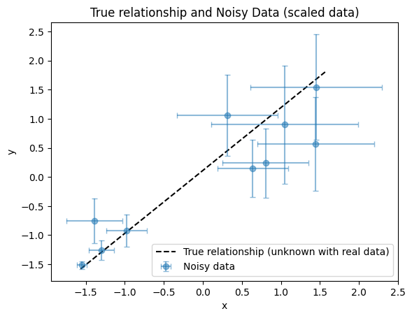
We use the helper function to generate synthetic noisy data, noting that errors in the \(x\) variable are now included.

x_true, x_obs, y_true, y_obs = generate_linear_data(
    m=true_slope,
    c=true_intercept,
    num=num,
    x_range=x_range,
    x_noise_std=x_noise_std,
    y_noise_std=y_noise_std,
)

We perform data scaling and plot the result.

data_scaler = DataScaler(x_true, y_obs)

x_true_scaled = data_scaler.transform_x(x_true)
y_true_scaled = data_scaler.transform_y(y_true)
x_obs_scaled, x_noise_std_scaled = data_scaler.transform_x(x_obs, x_noise_std)
y_obs_scaled, y_noise_std_scaled = data_scaler.transform_y(y_obs, y_noise_std)

plot_true_relationship_and_noisy_data(
    x_true_scaled,
    y_true_scaled,
    y_obs_scaled,
    y_noise_std_scaled,
    suffix="(scaled data)",
    x_obs=x_obs_scaled,
    x_noise_std=x_noise_std_scaled,
)

(<Figure size 640x480 with 1 Axes>,
 <Axes: title={'center': 'True relationship and Noisy Data (scaled data)'}, xlabel='x', ylabel='y'>)

4.3. Slope and intercept estimation

We set up the Bayesian parameter estimation model similar to before, but with two important additions. Focus on the big-picture concepts:

1. We do not know the true \(x\) values; we only know that each is likely to be close to its observed value, within the range set by its error bar (which can differ for each point). Therefore, we treat the true \(x\) values as latent variables—quantities that affect the model but are not directly observed. An important advantage of this approach is that our model will provide estimates of the true \(x\) values!

2. We must include a likelihood term for the observed \(x\) values, which tells us how plausible the observed \(x\) is, given the latent true \(x\) and its uncertainty. This allows the model to account for measurement error in both \(x\) and \(y\) in a principled way.

with pm.Model() as model:
    # Priors: Allow the slope and intercept to take a wide range of possible values
    slope = pm.Uniform("slope", lower=-3, upper=3)
    intercept = pm.Uniform("intercept", lower=-3, upper=3)

    # New compared to the model without x noise
    # Prior (for latent variable): For each data point, we assign a prior distribution to the true
    # (latent) x value. In this case, the prior is "data-informed": it is a normal distribution
    # centered on the observed x value, with its measurement error as the standard deviation. This
    # reflects our uncertainty about the true x before considering the y data, and is sometimes
    # called a measurement model or error model in Bayesian statistics.
    x_true_latent = pm.Normal(
        "x_true_latent", mu=x_obs_scaled, sigma=x_noise_std_scaled, shape=len(x_obs_scaled)
    )

    # Model: Use the estimated true x values to define the expected y values according to a
    # straight-line relationship
    mu = slope * x_true_latent + intercept

    # Likelihood: How well do the estimated true x values explain the observed x values?
    x_obs = pm.Normal("x_obs", mu=x_true_latent, sigma=x_noise_std_scaled, observed=x_obs_scaled)

    # Likelihood: How well do the expected y values explain the observed y values?
    y_obs = pm.Normal("y_obs", mu=mu, sigma=y_noise_std_scaled, observed=y_obs_scaled)

    # Sample from the posterior distribution using MCMC to find parameter values that best explain
    # the observed data
    idata = pm.sample(2000, tune=1000, return_inferencedata=True, random_seed=42)

Initializing NUTS using jitter+adapt_diag...
Sequential sampling (2 chains in 1 job)
NUTS: [slope, intercept, x_true_latent]

/home/docs/checkouts/readthedocs.org/user_builds/learn-data/envs/latest/lib/python3.13/site-packages/rich/live.py:2
60: UserWarning: install "ipywidgets" for Jupyter support
  warnings.warn('install "ipywidgets" for Jupyter support')

Sampling 2 chains for 1_000 tune and 2_000 draw iterations (2_000 + 4_000 draws total) took 9 seconds.
We recommend running at least 4 chains for robust computation of convergence diagnostics

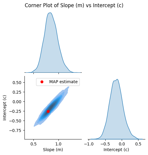
We calculate and display the MAP estimate for the slope and intercept.

# Extract samples for slope and intercept
m_samples = idata["posterior"]["slope"].stack(samples=("chain", "draw")).values
c_samples = idata["posterior"]["intercept"].stack(samples=("chain", "draw")).values

map_m, map_c = joint_map_estimate(m_samples, c_samples)

print(f"Single MAP estimate: Slope (m) = {map_m:.4f}, Intercept (c) = {map_c:.4f}")

Single MAP estimate: Slope (m) = 0.7902, Intercept (c) = -0.2601

4.4. Plotting

Visualize the joint distribution of slope and intercept.

g = plot_corner(m_samples, c_samples)

# Plot the MAP estimate on the lower left plot
ax = g.axes[1, 0]
ax.plot(map_m, map_c, "ro", label="MAP estimate")
ax.legend()

<matplotlib.legend.Legend at 0x7975db1e8690>

Recall that through construction of our model, we now also have samples for each true (latent) \(x\) value. By summarizing these samples with the median for each point, we obtain a robust estimate of the most probable true \(x\) positions. The median is commonly used because it is straightforward to compute and less sensitive to outliers than the mean, while being easier to evaluate than the mode for continuous samples. This provides a practical and interpretable way to evaluate and plot the best-fit regression line, while acknowledging the uncertainty in \(x\). However, it is important to recognize that summarizing the true \(x\) value in this way necessarily collapses one dimension of the uncertainty, potentially underrepresenting the full variability in the true \(x\) values.

x_true_latent_samples = idata["posterior"]["x_true_latent"].stack(samples=("chain", "draw")).values
x_true_median = np.median(x_true_latent_samples, axis=-1)

print("Median of latent x samples (best guess for true x values):", x_true_median)

Median of latent x samples (best guess for true x values): [-1.56138287 -1.30144174 -0.95480495 -1.22385226  0.57781292  0.71735987
  0.56262813  1.3089577   1.58674585  1.07312531]

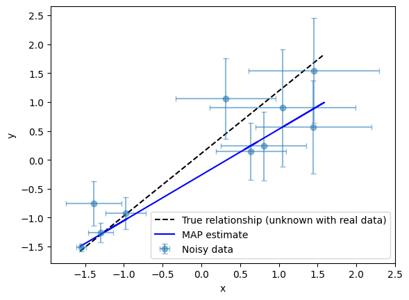
We compare the regression results visually.

fig, ax = plot_true_relationship_and_noisy_data(
    x_true_scaled,
    y_true_scaled,
    y_obs_scaled,
    y_noise_std_scaled,
    x_obs=x_obs_scaled,
    x_noise_std=x_noise_std_scaled,
)

# Add MAP fit line
# Note: We use the median of the latent x samples as our best guess for the true x values
y_map_fit = x_true_median * map_m + map_c
ax.plot(x_true_median, y_map_fit, "b-", label="MAP estimate")

ax.legend()  # Update legend

<matplotlib.legend.Legend at 0x7975db123890>

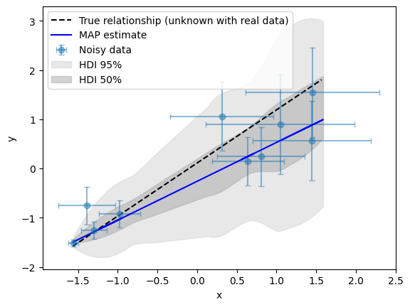
We generate new predicted observations from the model:

with model:
    pm.sample_posterior_predictive(idata, extend_inferencedata=True)

Sampling: [x_obs, y_obs]

/home/docs/checkouts/readthedocs.org/user_builds/learn-data/envs/latest/lib/python3.13/site-packages/rich/live.py:2
60: UserWarning: install "ipywidgets" for Jupyter support
  warnings.warn('install "ipywidgets" for Jupyter support')

We plot the linear relationship with the HDI regions.

y_pp = idata["posterior_predictive"]["y_obs"].values

fig, ax = plot_true_relationship_and_noisy_data(
    x_true_scaled,
    y_true_scaled,
    y_obs_scaled,
    y_noise_std_scaled,
    x_obs=x_obs_scaled,
    x_noise_std=x_noise_std_scaled,
)

# Add MAP fit line
y_map_fit = x_true_median * map_m + map_c
ax.plot(x_true_median, y_map_fit, "b-", label="MAP estimate")

# Plot the HDI regions
az.plot_hdi(
    x_true_median, y_pp, hdi_prob=0.95, fill_kwargs={"alpha": 0.5, "color": "lightgrey"}, ax=ax
)
az.plot_hdi(
    x_true_median, y_pp, hdi_prob=0.5, fill_kwargs={"alpha": 0.5, "color": "darkgrey"}, ax=ax
)

# Manually add legend entries for HDI regions
handles, labels = ax.get_legend_handles_labels()
hdi_95_patch = mpatches.Patch(color="lightgrey", alpha=0.5, label="HDI 95%")
hdi_50_patch = mpatches.Patch(color="darkgrey", alpha=0.5, label="HDI 50%")
handles += [hdi_95_patch, hdi_50_patch]
labels += ["HDI 95%", "HDI 50%"]

ax.legend(handles=handles)  # Update legend with HDI entries

<matplotlib.legend.Legend at 0x7975db1a3250>

4.5. Summary

Estimating fitting parameters from data with both \(x\) and \(y\) noise is our first substantial application of Bayesian estimation to a problem that cannot be addressed by traditional OLS or WLS approaches, which require a (relatively) noise-free predictor variable \(x\). Although reaching this point has required us to skip over some details, we now have a practical workflow for tackling a common challenge in scientific research.

This example demonstrates that Bayesian estimation:

• can be applied to data sets with known or estimated noise in any or all variables, as shown here for both the predictor (\(x\)) and response (\(y\)) variables.

• can estimate “latent” variables in the system, such as the true \(x\) values, which are not precisely known from the data and must be inferred as part of the Bayesian model.

• can provide a comprehensive picture of parameter uncertainties.