3. Bayesian Parameter Estimation I

# SPDX-FileCopyrightText: 2026 Dan J. Bower <dbower@eaps.ethz.ch>
#
# SPDX-License-Identifier: GPL-3.0-or-later

import arviz as az
import matplotlib.patches as mpatches
import numpy as np
import pymc as pm

from learn_data.regression import (
    DataScaler,
    generate_linear_data,
    joint_map_estimate,
    plot_corner,
    plot_true_relationship_and_noisy_data,
)

3.1. Learning objectives

1. Apply Bayesian parameter estimation to a dataset with heteroscedastic noise in the \(y\) variable

2. Understand the difference between using Bayesian parameter estimation on a single dataset compared to a frequentist approach that averages parameter estimates over many simulated datasets with different noise realizations

3.2. Introduction

So far, we have explored the classical approaches to regression using ordinary least-squares (OLS) and weighted least-squares (WLS), and shown how these methods can be extended with sampling to generate statistical distributions for parameters and their uncertainties. This naturally raises several question: can this workflow be generalized? What if we want to fit a relationship that is not linear? What if our model has more parameters? What if there are uncertainties in \(x\) as well as \(y\)? As the complexity and realism of our problems increases, the simple assumptions and frameworks of OLS and WLS often become inadequate or less effective.

To move forward, it’s helpful to shift our perspective. While we often talk about “fitting data,” in practice, the real goal in science is to estimate the values of underlying parameters that best explain the data, along with their uncertainties. As we’ve seen, sampling approaches allow us to estimate both the parameter values and their uncertainties directly from data. Thus, it’s more useful to think of the true objective as “estimating parameters from data” rather than “fitting parameters to data.”

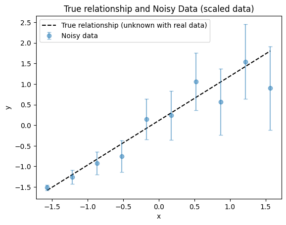
As before, let’s generate some noisy data, following the same noise model for the \(y\) variable as the WLS lecture.

# Define the parameters for the linear data generation. This is the "true" underlying relationship
# that we will try to recover using Bayesian parameter estimation.
true_slope = 1  # slope
true_intercept = 1.5  # intercept
num = 10  # number of data points
x_range = (0, 5)  # range of x values for data generation
y_noise_std = np.linspace(0.1, 1.5, num=num)  # Linearly increasing noise standard deviation

We use the helper function to generate synthetic noisy data

x_true, _, y_true, y_obs = generate_linear_data(
    m=true_slope, c=true_intercept, num=num, x_range=x_range, y_noise_std=y_noise_std
)

and perform data scaling.

data_scaler = DataScaler(x_true, y_obs)

x_true_scaled = data_scaler.transform_x(x_true)
y_true_scaled = data_scaler.transform_y(y_true)
y_obs_scaled, y_noise_std_scaled = data_scaler.transform_y(y_obs, y_noise_std)

plot_true_relationship_and_noisy_data(
    x_true_scaled, y_true_scaled, y_obs_scaled, y_noise_std_scaled, suffix="(scaled data)"
)

(<Figure size 640x480 with 1 Axes>,
 <Axes: title={'center': 'True relationship and Noisy Data (scaled data)'}, xlabel='x', ylabel='y'>)

It is helpful to know the true parameters in both original and scaled units.

true_slope_scaled, true_intercept_scaled = data_scaler.original_parameters_to_scaled(
    true_slope, true_intercept
)
print(f"True parameters: slope = {true_slope}, intercept = {true_intercept}")
print(f"Scaled true parameters: slope = {true_slope_scaled}, intercept = {true_intercept_scaled}")

True parameters: slope = 1, intercept = 1.5
Scaled true parameters: slope = [1.08029968], intercept = [0.11173754]

3.3. Slope and intercept estimation

If we shift our thinking to “estimating parameters”, it becomes clear that the slope and intercept should be the main focus of our analysis. It’s helpful to start with a reasonable idea of what these parameters could be. For example, we might expect them to fall within a certain range, centered around zero, so that both positive and negative values are equally possible. In Bayesian statistics, this initial idea about what values the parameters could take is called a prior. So, even if we don’t worry about the details yet, we are already introducing the correct terminology: we define priors for the slope and intercept.

For any given combination of slope and intercept, we can ask how well that combination produces a line that fits the data. In Bayesian statistics, this idea of measuring how well the parameters explain the observed data is called the likelihood. Without worrying about the technical details for now, just know that the likelihood tells us how plausible the data are for different parameter values. By systematically exploring many different parameter combinations (from the prior) and evaluating how well each one explains the observed data (the likelihood), we can identify which parameter values are preferred by our model. This process allows us to quantify our confidence in different parameter values, rather than just picking a single “best” answer.

with pm.Model() as model:
    # Define the prior distributions for the slope and intercept parameters.
    # Here, both slope and intercept are given uniform priors between -3 and 3.
    slope = pm.Uniform("slope", lower=-3, upper=3)
    intercept = pm.Uniform("intercept", lower=-3, upper=3)

    # The expected value of y for each x, given the parameters (the model).
    # This is just a linear model: y = mx + c, where m is the slope and c is the intercept.
    mu = slope * x_true_scaled + intercept

    # Define the likelihood: how likely the observed data are, given the model parameters.
    # We assume the observed y values are normally distributed around mu, with standard deviation
    # y_noise_std_scaled.
    y_obs = pm.Normal("y_obs", mu=mu, sigma=y_noise_std_scaled, observed=y_obs_scaled)

    # Sample from the posterior distribution using MCMC.
    idata = pm.sample(2000, tune=1000, return_inferencedata=True, random_seed=42)

Initializing NUTS using jitter+adapt_diag...
Sequential sampling (2 chains in 1 job)
NUTS: [slope, intercept]

/home/docs/checkouts/readthedocs.org/user_builds/learn-data/envs/latest/lib/python3.13/site-packages/rich/live.py:2
60: UserWarning: install "ipywidgets" for Jupyter support
  warnings.warn('install "ipywidgets" for Jupyter support')

Sampling 2 chains for 1_000 tune and 2_000 draw iterations (2_000 + 4_000 draws total) took 4 seconds.
We recommend running at least 4 chains for robust computation of convergence diagnostics

We extract the samples of the slope and intercept from the sampling process and compute the MAP.

# Extract samples for slope and intercept
m_samples = idata["posterior"]["slope"].stack(samples=("chain", "draw")).values
c_samples = idata["posterior"]["intercept"].stack(samples=("chain", "draw")).values

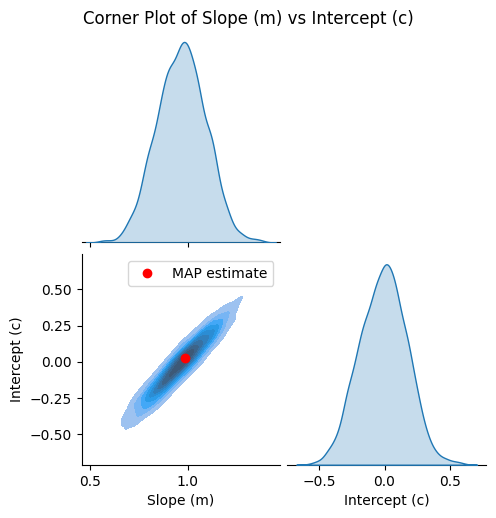
map_m, map_c = joint_map_estimate(m_samples, c_samples)

print(f"MAP estimate: Slope (m) = {map_m:.4f}, Intercept (c) = {map_c:.4f}")

MAP estimate: Slope (m) = 0.9880, Intercept (c) = 0.0242

We plot the corner plot

g = plot_corner(m_samples, c_samples)

# Plot the MAP estimate on the lower left plot
ax = g.axes[1, 0]
ax.plot(map_m, map_c, "ro", label="MAP estimate")
ax.legend()

<matplotlib.legend.Legend at 0x742891718550>

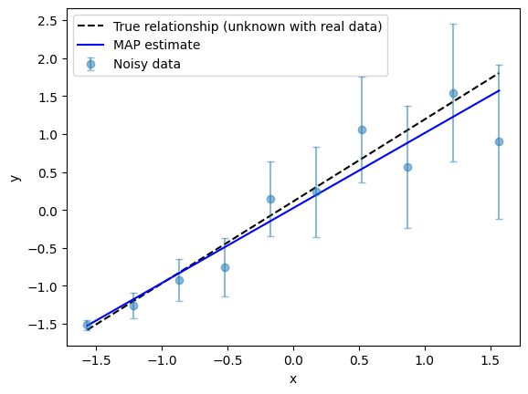
and compare the regression result visually.

fig, ax = plot_true_relationship_and_noisy_data(
    x_true_scaled, y_true_scaled, y_obs_scaled, y_noise_std_scaled
)

# Add MAP fit line
y_map_fit = x_true_scaled * map_m + map_c  # type: ignore
ax.plot(x_true_scaled, y_map_fit, "b-", label="MAP estimate")

ax.legend()  # Update legend

<matplotlib.legend.Legend at 0x742891747110>

3.4. Highest Density Interval (HDI)

So far, we’ve talked about uncertainty, but we’ve mostly focused on a single best-fit metric, the MAP estimate. However, the real strength of Bayesian methods is that they give us a whole range of possible answers, not just one.

In this regard, we can use our model to generate new data that are consistent with what we’ve learned from the actual data. This means we can see not just what is most likely, but also what other outcomes are possible and how likely they are.

To do this, we introduce the concept of the Highest Density Interval (HDI). Think of the HDI as the range where the model says the answer is most likely to be. For example, the 50% HDI is the narrowest range that contains the middle half of all the most likely predictions. The 95% HDI is a wider range that covers almost all the likely predictions. We can choose which HDIs to plot, depending on what is most useful for our problem and interpretation.

Don’t worry about the code snippet for now; we’ll explain exactly how it works later. For now, just remember that this command is used to generate new predicted observations from the model:

with model:
    pm.sample_posterior_predictive(idata, extend_inferencedata=True)

Sampling: [y_obs]

/home/docs/checkouts/readthedocs.org/user_builds/learn-data/envs/latest/lib/python3.13/site-packages/rich/live.py:2
60: UserWarning: install "ipywidgets" for Jupyter support
  warnings.warn('install "ipywidgets" for Jupyter support')

We plot the linear relationship with the HDI regions.

y_pp = idata["posterior_predictive"]["y_obs"].values

fig, ax = plot_true_relationship_and_noisy_data(
    x_true_scaled, y_true_scaled, y_obs_scaled, y_noise_std_scaled
)

# Add MAP fit line
y_map_fit = x_true_scaled * map_m + map_c  # type: ignore
ax.plot(x_true_scaled, y_map_fit, "b-", label="MAP estimate")

# Plot the HDI regions
az.plot_hdi(
    x_true_scaled, y_pp, hdi_prob=0.95, fill_kwargs={"alpha": 0.5, "color": "lightgrey"}, ax=ax
)
az.plot_hdi(
    x_true_scaled, y_pp, hdi_prob=0.5, fill_kwargs={"alpha": 0.5, "color": "darkgrey"}, ax=ax
)

# Manually add legend entries for HDI regions
handles, labels = ax.get_legend_handles_labels()
hdi_95_patch = mpatches.Patch(color="lightgrey", alpha=0.5, label="HDI 95%")
hdi_50_patch = mpatches.Patch(color="darkgrey", alpha=0.5, label="HDI 50%")
handles += [hdi_95_patch, hdi_50_patch]
labels += ["HDI 95%", "HDI 50%"]

ax.legend(handles=handles)  # Update legend with HDI entries

<matplotlib.legend.Legend at 0x742894f06210>

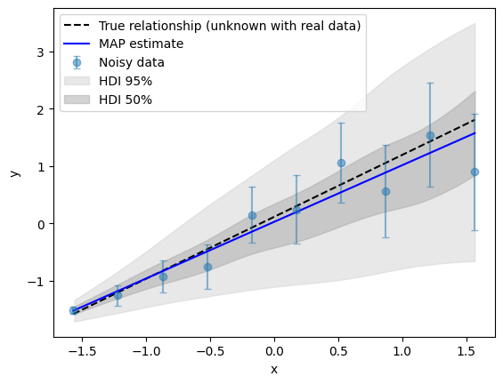
The dark grey region shows where 50% of the predicted data from our model are most likely to fall (the 50% HDI). The light grey region shows where 95% of the predictions are likely to fall (the 95% HDI). For this simple model, the MAP estimate is located near the center of the HDI regions. However, in general this is not always the case. As we would expect from the noisy data, the uncertainty bounds, given by the HDI regions, increase with \(x\).

In this example, the true relationship (the original line we used to generate the data) is recovered within the Bayesian model, to within a statistical bound. In fact, the true value falls within the 30% HDI, meaning it is among the most credible 30% of possible outcomes according to the model. The smaller the HDI that contains a value, the more strongly the model supports it as a likely outcome.

We note that 30% HDI is not just any 30% of the probability, but the most concentrated 30%—the region where the model thinks the answer is densest and most credible, even if not at the very center.

3.5. Fit comparison

It’s natural to wonder how the Bayesian fit compares to the WLS fit from the previous lecture. The fairest comparison is between the “Single WLS fit” from before and the “MAP estimate” here, since both utilize the information content of a single data set. For this linear fitting example, the slope and intercept values are in good agreement, even if not exactly the same. This is reasonable, as the underlying methods are different (we’ll discuss these differences in future lectures). Agreement is expected under certain conditions, but differences can arise depending on the data and assumptions. At this stage, the main point is to show that Bayesian estimation can recover results similar to those from more familiar approaches like WLS.

However, as revealed by the previous figure, the key point is that Bayesian estimation provides richer information: it gives not only estimates of the slope and intercept, but also their uncertainties. Furthermore, a real strength of Bayesian estimation is its flexibility: it can be applied to much more complex problems, which are common in real scientific work. While OLS and WLS are simple and fast, they rely on specific assumptions, for example about the noise model. Bayesian estimation, on the other hand, can handle a wider range of situations and uncertainties, making it a powerful tool as problems become more realistic and challenging.

3.6. Parameter estimation on real and simulated data

There are two main ways parameter estimation is used:

1. On real data: Usually, we have only one dataset. Bayesian estimation is used to answer: ‘Given the data I actually observed, what can I say about the parameters?’ The result is the best possible inference for the data at hand, along with a description of uncertainty that reflects what we can learn from those specific measurements.

2. On simulated data (noise simulation): When testing or comparing methods, researchers may generate many simulated datasets with different noise realizations. We introduced this approach in previous lectures using OLS and WLS. By applying OLS/WLS to each simulated dataset and then averaging the results, we can see how well a method recovers the true parameters on average. This helps us understand the typical performance, bias, or variability of a method.

Both approaches are useful: simulation studies help us understand the general behavior of a method, while Bayesian estimation on real data tells us what we can say about the parameters given the measurements we actually have. So, if the Bayesian estimate for this simple linear model doesn’t match the true relationship as closely as the average WLS result using Monte Carlo sampling, that’s expected. This is because we know the noise model exactly and can use repeated sampling to average out random fluctuations.

However, Bayesian estimation becomes especially valuable when the noise model is uncertain, the data are limited, or the model is more complex or hierarchical. Bayesian methods provide a principled way to quantify uncertainty and incorporate prior knowledge, making them more flexible and robust for real-world scientific problems.

3.7. Summary

• Bayesian parameter estimation can be used to perform linear regression and is compatible with results obtained from more familiar techniques such as weighted least squares.

• Bayesian approaches are designed to operate on a single dataset, providing a complete picture of what that dataset can imply about model parameters and their uncertainties.

• With the Bayesian framework introduced here, subsequent lectures will extend these ideas to problems frequently encountered in scientific applications.