2. Weighted Least Squares

# SPDX-FileCopyrightText: 2026 Dan J. Bower <dbower@eaps.ethz.ch>
#
# SPDX-License-Identifier: GPL-3.0-or-later

import matplotlib.pyplot as plt
import numpy as np
from sklearn.linear_model import LinearRegression

from learn_data.regression import (
    DataScaler,
    generate_linear_data,
    joint_map_estimate,
    plot_corner,
    plot_true_relationship_and_noisy_data,
)

2.1. Learning objectives

1. Use weighted least-squares for variable errors in the response variable (\(y\)).

2. Combine WLS with Monte Carlo simulation to propagate uncertainty in the dependent variable \(y\).

2.2. Introduction

In scientific data, it is common to encounter situations where each data point has a different level of uncertainty or noise. This means the strict assumption of constant variance (homoscedasticity) made by ordinary least squares (OLS) is often violated. When the noise level varies from point to point (heteroscedasticity), OLS is no longer optimal. Weighted least squares (WLS) provides a way forward by allowing us to account for these variable uncertainties, assigning more weight to data points with lower noise and less weight to those with higher noise.

In effect, WLS transforms the regression problem so that, after weighting, the transformed residuals have approximately constant variance, restoring the conditions under which least squares estimation is statistically efficient.

As before, let’s generate noisy data from a linear relationship, but this time each data point in \(y\) will have its own noise scale. This simulates heteroscedasticity, where the variance of the errors varies across observations. We impose a noise scale that increases with \(x\) to facilitate understanding, but WLS works with any heteroscedasticity.

# Parameters for the true linear relationship. This is the "ground truth" that we will try to
# recover through regression.
true_slope = 1  # slope
true_intercept = 1.5  # intercept
num = 10  # number of data points
x_range = (0, 5)  # range of x values for data generation
y_noise_std = np.linspace(0.1, 1.5, num=num)  # linearly increasing noise standard deviation

We us the helper function to generate synthetic noisy data.

x_true, _, y_true, y_obs = generate_linear_data(
    m=true_slope, c=true_intercept, num=num, x_range=x_range, y_noise_std=y_noise_std
)

We perform data scaling and plot the relationship.

data_scaler = DataScaler(x_true, y_obs)

x_true_scaled = data_scaler.transform_x(x_true)
y_true_scaled = data_scaler.transform_y(y_true)
y_obs_scaled, y_noise_std_scaled = data_scaler.transform_y(y_obs, y_noise_std)

plot_true_relationship_and_noisy_data(
    x_true_scaled, y_true_scaled, y_obs_scaled, y_noise_std_scaled, suffix="(scaled data)"
)

(<Figure size 640x480 with 1 Axes>,
 <Axes: title={'center': 'True relationship and Noisy Data (scaled data)'}, xlabel='x', ylabel='y'>)

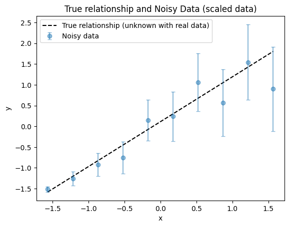
It is helpful to know the true parameters in both original and scaled units.

true_slope_scaled, true_intercept_scaled = data_scaler.original_parameters_to_scaled(
    true_slope, true_intercept
)
print(f"True parameters: slope = {true_slope}, intercept = {true_intercept}")
print(f"Scaled true parameters: slope = {true_slope_scaled}, intercept = {true_intercept_scaled}")

True parameters: slope = 1, intercept = 1.5
Scaled true parameters: slope = [1.08029968], intercept = [0.11173754]

2.3. WLS regression

What is WLS?

WLS is a way to fit a straight line to data when the variability (uncertainty) of each data point is not the same. Instead of treating all points equally, WLS gives more importance (weight) to points with smaller errors and less importance to points with larger errors. This means the best-fit line is influenced more by the most reliable data.

Mathematically, WLS works by minimizing the sum of the squared residuals, but each residual is divided by the variance (or squared uncertainty) of its data point. This way, points with higher uncertainty contribute less to the total error.

Why do we use WLS?

• It gives the most accurate fit when the data points have different uncertainties.

• It prevents noisy (less reliable) points from having too much influence on the fit.

• It is essential in scientific and engineering applications where measurement errors are not uniform.

What does WLS assume?

• The same assumptions as OLS, except relaxing the requirement for a constant noise level for all response variables (\(y\)).

How realistic are these assumptions for real data?

In practice, WLS is especially useful when you know or can estimate the uncertainty for each measurement. This is common in experiments where each observation comes with its own error bar. However, if the uncertainties are not known or are estimated poorly, the results can be misleading.

WLS is widely used in science and engineering because it allows you to make the most of your data, even when some points are much more precise (less noisy) than others.

Now we can perform WLS regression and obtain the slope and intercept.

# Reshape x_scaled for sklearn (expects 2D array)
x_true_scaled_reshaped = x_true_scaled.reshape(-1, 1)  # type: ignore

# Fit WLS regression model
reg = LinearRegression()
reg.fit(x_true_scaled_reshaped, y_obs_scaled, sample_weight=1 / y_noise_std_scaled**2)

# Get slope and intercept
wls_slope = reg.coef_
wls_intercept = reg.intercept_

print(f"WLS slope: {wls_slope[0]:.4f}, WLS intercept: {wls_intercept:.4f}")

WLS slope: 0.9676, WLS intercept: -0.0106

We plot the WLS regression.

fig, ax = plot_true_relationship_and_noisy_data(
    x_true_scaled, y_true_scaled, y_obs_scaled, y_noise_std_scaled, suffix="(scaled data)"
)
# Add WLS solution
ax.plot(x_true_scaled, reg.predict(x_true_scaled_reshaped), "b-", label="Single WLS fit")
ax.legend()  # Re-add legend to include WLS fit

<matplotlib.legend.Legend at 0x70c91fce4190>

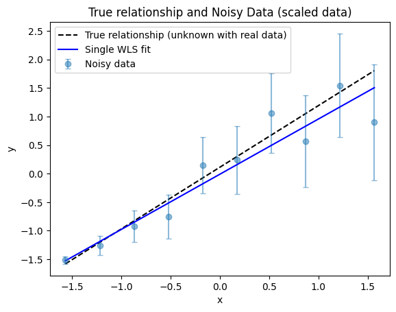
2.3.1. Fit comparison

It is clear from the plot that the WLS fit gives more weight to the more reliable data points—those with smaller uncertainties, which in this example correspond to the smaller \(x\) values. Conversely, the WLS fit is less influenced by the data points with larger uncertainties at higher \(x\) values, so the fitted line is not “pulled” toward these noisier points.

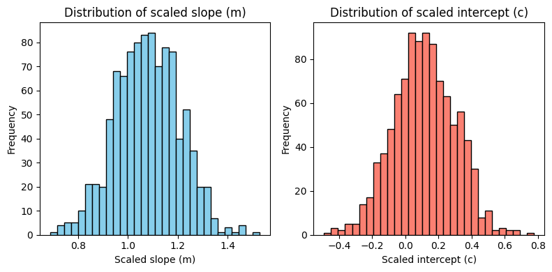
2.4. Uncertainty propagation

By using Monte Carlo sampling to generate many realizations of the data with different noise, we can compute statistics over the resulting population of fits.

n_samples = 1000  # Number of Monte Carlo samples
m_samples_list = []
c_samples_list = []

# Create the regression once outside the loop to avoid re-initializing it every iteration
reg_mc = LinearRegression()

for _ in range(n_samples):
    # Generate new y_sample using the same x and the helper function for consistency
    _, _, _, y_sample = generate_linear_data(
        m=true_slope, c=true_intercept, num=num, x_range=x_range, y_noise_std=y_noise_std
    )
    # Scale the resampled y using the same scaler as before
    y_sample_scaled = data_scaler.transform_y(y_sample)

    # Fit regression on scaled data with noise-based weights
    reg_mc.fit(
        x_true_scaled_reshaped,
        y_sample_scaled.reshape(-1, 1),  # type: ignore
        # Specify the weights as the inverse of the variance (1 / std^2) for WLS
        sample_weight=1 / y_noise_std_scaled**2,
    )
    m_samples_list.append(reg_mc.coef_)
    c_samples_list.append(reg_mc.intercept_)

m_samples = np.array(m_samples_list).flatten()
c_samples = np.array(c_samples_list).flatten()

We now plot the distributions of the fitted slope (\(m\)) and intercept (\(c\)) values obtained from the Monte Carlo simulations. These plots show the marginal distributions of each parameter.

fig, axes = plt.subplots(1, 2, figsize=(8, 4))

# Histogram for m_samples (slope)
axes[0].hist(m_samples, bins=30, color="skyblue", edgecolor="black")
axes[0].set_title("Distribution of scaled slope (m)")
axes[0].set_xlabel("Scaled slope (m)")
axes[0].set_ylabel("Frequency")

# Histogram for c_samples (intercept)
axes[1].hist(c_samples, bins=30, color="salmon", edgecolor="black")
axes[1].set_title("Distribution of scaled intercept (c)")
axes[1].set_xlabel("Scaled intercept (c)")
axes[1].set_ylabel("Frequency")

plt.tight_layout()

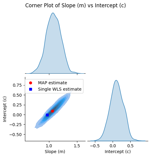
We calculate the maximum a posteriori (MAP) estimate as described in the OLS lecture.

map_m, map_c = joint_map_estimate(m_samples, c_samples)

print(f"MAP estimate: Slope (m) = {map_m:.4f}, Intercept (c) = {map_c:.4f}")

MAP estimate: Slope (m) = 1.0596, Intercept (c) = 0.0956

We plot the corner plot

g = plot_corner(m_samples, c_samples)

# Plot the MAP estimate on the lower left plot
ax = g.axes[1, 0]
ax.plot(map_m, map_c, "ro", label="MAP estimate")
ax.plot(wls_slope, wls_intercept, "bs", label="Single WLS estimate")
ax.legend()

<matplotlib.legend.Legend at 0x70c91d7ef9d0>

and compare the regression results visually.

fig, ax = plot_true_relationship_and_noisy_data(
    x_true_scaled, y_true_scaled, y_obs_scaled, y_noise_std_scaled
)

# add the WLS solution
ax.plot(x_true_scaled, reg.predict(x_true_scaled_reshaped), "b-", label="Single WLS fit")

# Add MAP fit line
y_map_fit = map_m * x_true_scaled + map_c  # type: ignore
ax.plot(x_true_scaled, y_map_fit, "g-", label="MAP fit")

ax.legend()  # Update legend

<matplotlib.legend.Legend at 0x70c91d66a5d0>

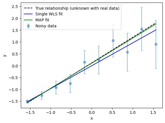
2.5. Summary

• Weight least-squares (WLS) extends the possibility of least-squares fitting to data with variable noise in response variables (\(y\)).

• As with OLS, WLS is simple to implement and computationally efficient.

• Combining WLS with Monte Carlo simulation permits uncertainty estimation on the parameters.