1. Ordinary Least Squares

# SPDX-FileCopyrightText: 2026 Dan J. Bower <dbower@eaps.ethz.ch>
#
# SPDX-License-Identifier: GPL-3.0-or-later

import matplotlib.pyplot as plt
import numpy as np
from sklearn.linear_model import LinearRegression

from learn_data.regression import (
    DataScaler,
    generate_linear_data,
    joint_map_estimate,
    plot_corner,
    plot_true_relationship_and_noisy_data,
)

Matplotlib is building the font cache; this may take a moment.

1.1. Learning objectives

1. Review and apply ordinary least squares (OLS) regression for data modeling.

2. Combine OLS with Monte Carlo simulation to propagate uncertainty in the dependent variable \(y\).

3. Interpret probabilistic outputs and uncertainty in model predictions using corner plots.

4. Extract point estimates from probability distributions.

1.2. Introduction

Regression analysis is a fundamental tool in science and engineering for understanding relationships between variables. It allows researchers to model and quantify how one or more predictor variables (\(x\)) influence a response variable (\(y\)), making it essential for prediction, uncertainty quantification, and data interpretation. Among various regression techniques, linear regression is especially common due to its simplicity, interpretability, and effectiveness in modeling linear relationships. It serves as a foundational method in statistics, machine learning, and many scientific disciplines.

In this lecture, we start with ordinary least squares (OLS) regression to introduce the basic concepts of fitting a line to data. We then use sampling techniques to estimate uncertainty in our model parameters. This approach naturally leads us toward a probabilistic perspective, where we can quantify uncertainty in a principled way.

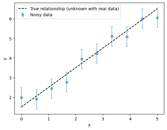
First, we generate synthetic data that adheres to a linear relationship. The function below generates data points that adhere to a linear relationship with Gaussian noise of 0.5 standard deviations added to the \(y\) values.

# Parameters for the true linear relationship. This is the "ground truth" that we will try to
# recover through regression.
true_slope = 1
true_intercept = 1.5
num = 10  # number of data points
x_range = (0, 5)  # range of x values for data generation
y_noise_std = 0.5  # standard deviation of noise in y values (must be > 0 for noisy data)

We use the helper function to generate synthetic noisy data.

x_true, _, y_true, y_obs = generate_linear_data(
    m=true_slope, c=true_intercept, num=num, x_range=x_range, y_noise_std=y_noise_std
)

It’s always a good first step to plot the raw data. Visualizing data before any analysis helps to quickly spot trends, patterns, outliers, or potential issues. This initial plot provides valuable intuition about the underlying relationships and guides choices of models and preprocessing steps. Of course, in real-world scenarios, the true underlying relationship is not known. Here, we plot it for completeness because this is a synthetic example where we have control over the data generation process.

plot_true_relationship_and_noisy_data(x_true, y_true, y_obs, y_noise_std)

(<Figure size 640x480 with 1 Axes>, <Axes: xlabel='x', ylabel='y'>)

1.3. Data scaling

Scaling the data means changing the values of your variables so that they all use a similar range or unit. This is important in regression and many machine learning algorithms because it ensures that all variables are treated fairly by the model.

Imagine you are comparing the heights of people (measured in meters) and their incomes (measured in CHF). If you don’t scale the data, the income numbers (which can be in the tens of thousands) will dominate the calculations, and the model might ignore the height variable just because its numbers are much smaller. This can lead to biased or misleading results.

To avoid this, we often standardize the data. Standardizing means adjusting each variable so that it has a mean (average) of 0 and a standard deviation (spread) of 1. After standardization, all variables are on the same scale, and the model can compare them more fairly.

Why is this helpful?

• It helps the model learn more efficiently and accurately.

• It prevents variables with large numbers from overpowering those with smaller numbers.

• It makes it easier to interpret the results, since all variables are measured in the same way in terms of how many standard deviations they are from the mean.

data_scaler = DataScaler(x_true, y_obs)

x_true_scaled = data_scaler.transform_x(x_true)
y_true_scaled = data_scaler.transform_y(y_true)
y_obs_scaled, y_noise_std_scaled = data_scaler.transform_y(y_obs, y_noise_std)

plot_true_relationship_and_noisy_data(
    x_true_scaled, y_true_scaled, y_obs_scaled, y_noise_std_scaled, suffix="(scaled data)"
)

(<Figure size 640x480 with 1 Axes>,
 <Axes: title={'center': 'True relationship and Noisy Data (scaled data)'}, xlabel='x', ylabel='y'>)

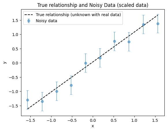
Once data have been transformed into scaled units, it is standard practice to keep all variables in these scaled units throughout the analysis. If needed, results can be converted back to the original units at the end for interpretation or publication. Therefore, it is helpful to know the true parameters in both original and scaled units. For a linear function, the transformation between original and scaled parameters is straightforward to derive.

true_slope_scaled, true_intercept_scaled = data_scaler.original_parameters_to_scaled(
    true_slope, true_intercept
)
print(f"True parameters: slope = {true_slope}, intercept = {true_intercept}")
print(f"Scaled true parameters: slope = {true_slope_scaled}, intercept = {true_intercept_scaled}")

True parameters: slope = 1, intercept = 1.5
Scaled true parameters: slope = [1.05076382], intercept = [0.03047314]

1.4. OLS regression

What is OLS?

OLS is a way to find the line that best fits a set of data points. Imagine you have a scatter plot of points, and you want to draw a straight line that goes as close as possible to all of them. OLS does this by finding the line that makes the vertical distances between the points and the line as small as possible, on average.

These vertical distances are called residuals—they show how far off each data point is from the line. OLS works by squaring each of these distances (so that negative and positive differences don’t cancel out), adding them all up, and then finding the line that makes this total as small as possible. That’s why it’s called “least squares.”

Why do we use OLS?

• It’s simple and works well for linear functions.

• It gives us a clear formula for the best-fit line, which we can use to make predictions.

• It’s the most common starting point for learning about regression and modeling data.

What does OLS assume?

• Predictor variables (\(x\)) are measured without error, or at least with negligible error compared to the response variable (\(y\)).

• The errors (differences between the actual \(y\) values and the values predicted by the line) are only in \(y\) (the response), not in \(x\) (the predictor).

• The errors are independent (one data point’s error doesn’t affect another’s).

• The errors are identically distributed: they all come from the same probability distribution (sometimes assumed normal, but normality is not required for the line to be the best fit), and have the same spread (variance) and shape.

• The relationship between predictor (\(x\)) and response variables (\(y\)) can be described by a function that is linear in its parameters (coefficients).

How realistic are these assumptions for real data?

It’s natural to wonder whether real-world data actually follows all these requirements. In practice, real data often only approximately meets these assumptions:

• Sometimes the relationship between predictors and responses cannot be represented by a function that is perfectly linear.

• Errors might not be perfectly independent (for example, measurements taken close together in time might be correlated).

• The spread (variance) of the errors might change for different values of \(x\) (this is called heteroscedasticity).

• Errors might not be exactly normally distributed.

However, OLS is still widely used because it is robust to small violations of these assumptions, especially with large datasets.

Note: There are also formal statistical tests and more advanced diagnostic tools (such as tests for normality, constant variance, and independence of errors) that can help you decide if OLS is appropriate for your data. In this introductory notebook, we focus on building intuition and using visual checks. We will cover these formal tests and diagnostics in more detail in a later notebook.

Now we can perform OLS regression and obtain the slope and intercept.

# Reshape x_scaled for sklearn (expects 2D array)
x_true_scaled_reshaped = x_true_scaled.reshape(-1, 1)  # type: ignore

# Fit linear regression model
reg = LinearRegression()
reg.fit(x_true_scaled_reshaped, y_obs_scaled)

# Get slope and intercept
ols_slope = reg.coef_
ols_intercept = reg.intercept_

print(f"OLS slope: {ols_slope[0]}, OLS intercept: {ols_intercept}")

OLS slope: 0.9837028775325071, OLS intercept: 1.7763568394002506e-16

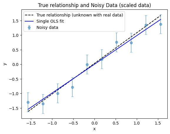
The recovered OLS intercept is essentially zero, which is expected because the data scaling procedure for \(y\) centers the data. Let’s now visualize the OLS regression result to see how well the fitted line matches the scaled data.

fig, ax = plot_true_relationship_and_noisy_data(
    x_true_scaled, y_true_scaled, y_obs_scaled, y_noise_std_scaled, suffix="(scaled data)"
)
# Add OLS result to the plot
ax.plot(x_true_scaled, reg.predict(x_true_scaled_reshaped), "b-", label="Single OLS fit")
ax.legend()  # Re-add legend to include OLS fit

<matplotlib.legend.Legend at 0x717247af4550>

1.4.1. Fit comparison

We notice that the OLS regression line diverges more from the true relationship at smaller \(x\) values than at larger \(x\) values. This might seem surprising, since the noise level is the same for all points. Why does the OLS regression match the true relationship better for some regions of \(x\) than for others?

This effect occurs because, even with constant noise, the random fluctuations in the data can align in such a way that the fitted line is pulled away from the true relationship in certain regions. With only a small number of data points, these random deviations can have a noticeable impact, especially at the edges of the data range. As a result, the OLS fit may appear to be better in some areas and worse in others, even though the noise is uniform across all points.

1.4.2. Does OLS depend on the noise scale?

Suppose we rerun the OLS regression, but this time we increase or decrease the noise scale (the standard deviation of the noise in \(y\)). We will find that the OLS solution (the best-fit slope and intercept) does not change.

Why is this?

• OLS regression does not explicitly include the noise scale in the optimization itself. Instead, it assumes that the errors are symmetric, independent, and identically distributed, treating all data points as equally reliable.

• OLS determines the best-fit parameters by minimizing the sum of squared residuals, without considering whether the overall noise level is large or small, provided the errors remain centered around zero.

• As a result, scaling the noise up or down does not change the location of the best-fit line itself.

Should this make us uncomfortable?

• In many situations, yes. Reporting only the OLS best-fit parameters ignores whether the data are highly noisy or extremely precise.

• OLS provides a single “best” solution, but by itself it does not quantify how uncertain that solution is.

• Put differently, the fitted line is insensitive to the absolute noise scale; only the estimated parameter uncertainties reflect it.

Capturing parameter uncertainty requires going beyond the basic OLS fit and propagating the noise through additional methods, as we will now discover.

1.5. Uncertainty propagation

Monte Carlo methods are a broad class of computational techniques that use random sampling to estimate the behavior of complex systems. The name comes from the famous casino in Monaco, reflecting the central role of randomness and probability in these methods.

In data analysis, Monte Carlo techniques are particularly valuable for uncertainty propagation. Rather than attempting to derive an exact analytical expression for how measurement errors affect the final result—which is often difficult or impossible—we instead generate many simulated versions of the dataset and analyze how the fitted parameters vary across those simulations.

Broadly speaking, there are two common approaches to estimating parameter uncertainties, which differ in how they model or resample noise in the data:

1. Parametric bootstrap (noise simulation). A noise model is assumed or estimated, and random noise is added to each data point according to that model. The perturbed dataset is then refitted. Repeating this process many times produces a distribution of fitted parameters.

2. Nonparametric bootstrap (resampling). Synthetic datasets are constructed by randomly resampling the original data, typically with replacement, meaning that original data points can appear more than once in the synthetic datasets. Each resampled dataset is refitted, allowing the variability of the fitted parameters to be estimated directly from the data itself.

In both approaches, the fitted parameters—for example, the slope and intercept in a linear regression—are recorded for every simulated dataset. The resulting collection of parameter estimates forms a statistical distribution, from which quantities such as means, standard deviations, and parameter correlations can be computed.

We will now extend our analysis to account for uncertainties (errors) in the response variable (\(y\)), while still assuming that our predictor variable (\(x\)) is known exactly. To estimate the impact of these errors on our regression parameters, we will use parametric boostrapping (noise simulations). This involves generating many synthetic datasets by sampling \(y\) according to its known error distribution, fitting the regression model to each dataset, and recording the resulting slope (\(m\)) and intercept (\(c\)) values. By analyzing the distributions of these fitted parameters, we can better understand their uncertainties and variability due to uncertainty in \(y\).

As we will see, this approach allows us to visualize how the noise scale influences the uncertainty in the estimated parameters, complementing OLS by moving beyond a single best-fit solution to a distribution of plausible fits.

n_samples = 1000  # Number of Monte Carlo samples
m_samples_list = []
c_samples_list = []

# Create the regression once outside the loop to avoid re-initializing it every iteration
reg_mc = LinearRegression()

for _ in range(n_samples):
    # Generate new y_sample using the same x and the helper function for consistency
    _, _, _, y_sample = generate_linear_data(
        m=true_slope, c=true_intercept, num=num, x_range=x_range, y_noise_std=y_noise_std
    )
    # Scale the resampled y using the same scaler as before
    y_sample_scaled = data_scaler.transform_y(y_sample)

    # Fit regression on scaled data and get slope and intercept
    reg_mc.fit(x_true_scaled_reshaped, y_sample_scaled.reshape(-1, 1))  # type: ignore

    # Save the parameter values for this sample
    m_samples_list.append(reg_mc.coef_)
    c_samples_list.append(reg_mc.intercept_)

m_samples = np.array(m_samples_list).flatten()
c_samples = np.array(c_samples_list).flatten()

We now plot the distributions of the fitted slope (\(m\)) and intercept (\(c\)) values obtained from the Monte Carlo simulations. These plots show the marginal distributions of each parameter.

fig, axes = plt.subplots(1, 2, figsize=(8, 4))

# Histogram for m_samples (slope)
axes[0].hist(m_samples, bins=30, color="skyblue", edgecolor="black")
axes[0].set_title("Distribution of slope (m)")
axes[0].set_xlabel("Slope (m)")
axes[0].set_ylabel("Frequency")

# Histogram for c_samples (intercept)
axes[1].hist(c_samples, bins=30, color="salmon", edgecolor="black")
axes[1].set_title("Distribution of intercept (c)")
axes[1].set_xlabel("Intercept (c)")
axes[1].set_ylabel("Frequency")

plt.tight_layout()

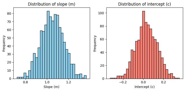
What is a marginal distribution?

Suppose you run the Monte Carlo simulation many times, each time getting a different value for the slope and intercept because of the random noise in the data. The marginal distribution for the slope (\(m\)) is a summary of how often you get each possible slope value, regardless of what the intercept was in that run. Similarly, the marginal distribution for the intercept (\(c\)) shows how likely each intercept value is, no matter what the slope was.

Why is this useful?

• It helps you see the range of plausible values for each parameter, given the measurement errors.

• A narrow distribution means you are confident about that parameter; a wide distribution means there is more uncertainty.

• By looking at these distributions, you can report not just a single “best” value, but also how much uncertainty there is in your estimates.

In summary: Marginal distributions help you understand how much the noise in your data affects your confidence in the slope and intercept values you report from your regression analysis.

1.6. Visualizing relationships

While the marginal distributions of \(m\) and \(c\) are useful for understanding the uncertainty in each parameter individually, they do not reveal the trade-off or correlation between the slope and intercept. Sometimes, the values of the slope and intercept are not independent: if you change one, you might need to change the other to still fit the data well. For example, a line with a steeper slope might need a lower intercept to pass through the same points. This relationship is called a correlation or trade-off between parameters.

A joint distribution (visualized in a corner plot or pair plot) shows how likely different combinations of slope and intercept are, based on your Monte Carlo simulations. Instead of just asking, “How likely is this slope?” or “How likely is this intercept?,” you ask, “How likely is it to get this slope and this intercept together?”

Why is this useful?

• It helps you see if there is a relationship between the two parameters (for example, if higher slopes tend to go with lower intercepts).

• It shows the most probable combinations of slope and intercept, not just their individual ranges.

• It gives a more complete picture of the uncertainty in your model, especially when parameters are not independent.

plot_corner(m_samples, c_samples)

<seaborn.axisgrid.PairGrid at 0x717247d64d70>

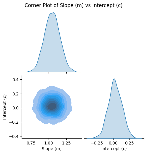
The pairplot above gives you a visual summary of what happened in all your Monte Carlo simulations. It shows both the individual (marginal) distributions for the slope (\(m\)) and intercept (\(c\)), and how these two parameters vary together (the joint distribution).

How do you read this plot?

• The diagonal plots (the ones along the top left to bottom right) show the marginal distributions for each parameter. These are like the histograms you saw earlier: they tell you how likely different values of the slope or intercept are, considering all the simulations.

• The off-diagonal plot (the lower-left corner) shows the joint distribution of \(m\) and \(c\). This is where you see how the two parameters are related. If the cloud of points or the contours are stretched out along a diagonal, it means that when the slope is higher, the intercept tends to be lower (or vice versa). This is a sign of a trade-off or correlation between the two parameters.

Note: When you standardize (scale) both \(x\) and \(y\) to have mean 0 and standard deviation 1, as we did here, the correlation between slope and intercept can disappear in the scaled space. This is because the regression line is forced to pass through the origin in scaled coordinates, making the slope and intercept statistically independent. In contrast, in the original (unscaled) data, the mean of \(x\) is not zero, so changes in the slope require compensating changes in the intercept, resulting in a negative correlation. Standardization is a feature that can simplify the interpretation of regression parameters by removing this correlation.

What do the shapes and colors mean?

• The spread (width) of the distributions tells you how much uncertainty there is. A narrow shape means you are confident in that parameter; a wide shape means there is more uncertainty.

• The contours in the joint plot are like elevation lines on a map: they show where most of your simulation results landed. The darkest or most saturated regions are where the most likely combinations of slope and intercept are found.

• Lighter regions mean fewer simulations landed there, so those combinations are less likely.

Why is this helpful?

• You can see not just the most likely values, but also how much they can vary due to noise in your data.

• You can spot if there is a relationship between the parameters (for example, if changing one means you have to change the other to still fit the data well).

• It helps you communicate the uncertainty and possible trade-offs in your model to others.

1.7. Point estimates

From a probabilistic perspective, it is ideal to show or report metrics that capture the full complexity of the parameter distributions, or even the entire distribution itself. This provides a more complete and honest picture of the uncertainty and variability in your results. However, in practice, it is often necessary or convenient to summarize the key relationships using point estimates, which distill the distribution down to a single representative value for each parameter. Hence, when you fit a model to data, you often want to report a single “best” value for each parameter (like the slope and intercept of a line). But because of noise and uncertainty, there isn’t just one answer—there’s a whole range of possible values. Furthermore, we expect that some of the parameters are correlated. So, how do you pick one value to report?

One common way:

• Find the most likely combination of parameters, based on all your simulations. This is called the maximum a posteriori (MAP) estimate. It’s just a fancy way of saying: “Out of all the possible combinations, this is the one that shows up most often in our results.”

• You can also use other summaries, like the average (mean) or the middle value (median), but the MAP is often used because it points to the most probable answer.

The MAP estimate can be determined in different ways. You could find the mode of the marginal distribution for \(m\) (slope) or \(c\) (intercept) individually, or you could find the mode of the joint distribution of both parameters. For the most compatible and representative point estimate, it is generally best to use the mode of the joint distribution, as this reflects the most likely combination of parameters given the data and their correlation.

Why do this?

• It gives you a single, clear answer to report, even though you know there’s uncertainty.

• It helps others quickly see what your model predicts, while the full distribution shows the uncertainty.

# This function computes the MAP estimate by finding the mode of the joint posterior distribution of m and c.
map_m, map_c = joint_map_estimate(m_samples, c_samples)

print(f"MC MAP estimate: Slope (m) = {map_m:.4f}, Intercept (c) = {map_c:.4f}")

MC MAP estimate: Slope (m) = 1.0397, Intercept (c) = 0.0144

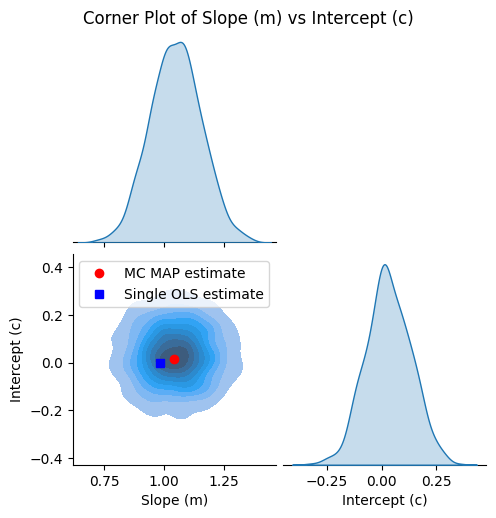
We re-plot the corner plot and also show the point estimates of the intercept and slope from the MAP and least-squares calculations.

g = plot_corner(m_samples, c_samples)

# Plot the MAP estimate on the lower left plot
ax = g.axes[1, 0]
ax.plot(map_m, map_c, "ro", label="MC MAP estimate")
ax.plot(ols_slope, ols_intercept, "bs", label="Single OLS estimate")
ax.legend()

<matplotlib.legend.Legend at 0x71724549e990>

Let’s also compare the regression results visually: we’ll plot both the linear fit using the MAP estimate and the single OLS fit.

fig, ax = plot_true_relationship_and_noisy_data(
    x_true_scaled, y_true_scaled, y_obs_scaled, y_noise_std_scaled
)

# Add OLS solution
ax.plot(x_true_scaled, reg.predict(x_true_scaled_reshaped), "b-", label="Single OLS fit")

# Add MAP fit line using the MAP estimates of slope and intercept
y_map_fit = map_m * x_true_scaled + map_c  # type: ignore
ax.plot(x_true_scaled, y_map_fit, "g-", label="MC MAP fit")

ax.legend()  # Update legend

<matplotlib.legend.Legend at 0x717245305590>

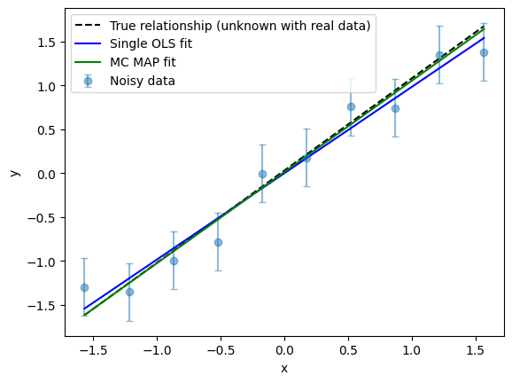
For this model at least, the MAP estimate of the slope and intercept from the MC sampling procedure produces a regression fit that more faithfully reproduces the original relationship.

Here’s why:

• A single OLS regression is influenced by the specific random noise in one dataset, which can cause its estimate to deviate from the true values. If you collected new data (or just had different random noise), you would likely get a different answer. So, the least-squares estimate is just one possible outcome among many.

• The MAP estimate, on the other hand, is found from MC sampling and represents the most probable parameter values across many noise realizations, effectively averaging out random fluctuations.

• Hence MC sampling tends to provide estimates that are less sensitive to outliers and more robust to random fluctuations, but it does not guarantee improved accuracy relative to the true parameters in every situation.

Note: Although analytical formulas exist for the standard errors (uncertainties) of the slope and intercept, they rely on specific assumptions—typically that the errors are independent, identically distributed, and normally distributed. In contrast, MC sampling offers a more flexible and general framework that can accommodate complex or realistic noise models. By simulating the data-generating process, MC provides an empirical way to estimate parameter uncertainty under a wide range of scenarios.

1.8. Summary

We have used the familiar concept of OLS regression as a foundation to introduce several important ideas that will be valuable as we move forward:

• Understanding and quantifying the uncertainty in parameters is crucial. One approach is to leverage sampling to generate many possible realizations of the data, allowing us to estimate the spread and reliability of our parameter estimates.

• Pairplots (corner plots) are powerful tools for visualizing both the uncertainty in parameters and the correlations or trade-offs between them. They help us see not just the range of plausible values, but also how parameters may be related.

• Point estimates, such as the MAP or mean, provide concise summaries of the most likely parameter values.

By combining these techniques, we move beyond simply reporting a single best-fit line and instead gain a deeper, more honest understanding of what our data and models are telling us.